Maybe at this point you’ve heard of AlphaZero and how it defeated Stockfish, which was then the best chess engine in the world. For those of you who haven’t, AlphaZero was a chess engine trained exclusively through self-play and deep learning. At this point it’s easy for us to look at Chess and think, “it’s still turn based and governed by strict rules, so the best chess engine being triumphed by another chess engine isn’t that exciting”. But what if I told you that AI was able to place in the top 0.2% in a popular real time strategy game like Starcraft, win against expert level players in Stratego, a game with bluffing and hidden information, and even score twice the points of the average player in a game with human negotiation like Diplomacy? All of these feats wouldn’t have been possible without help of neural networks, which are a huge contributor in allowing AI to make complex associations and decisions. Today I’ll be going over some of the basics.
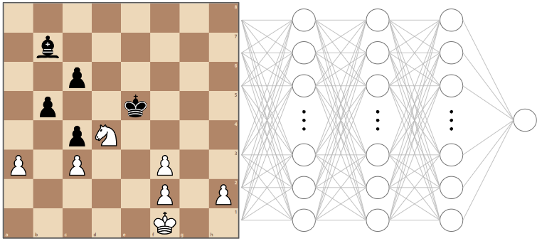
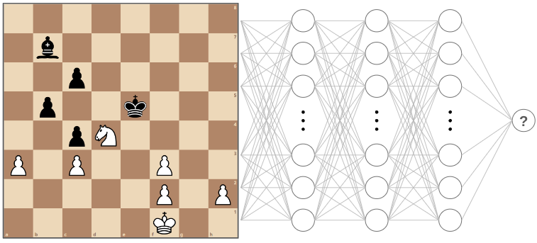
Below is a diagram of a neural network that outputs the evaluation on a chess position without performing any move analysis. This is known as a static evaluation.
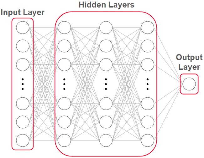
Each of these circles is called a neuron. The input layer consists of several neurons which receive the position of the board and other game information like castling rights and who’s turn to move it is. The output layer consists of one neuron, which returns the evaluation as a number. And the hidden layers are responsible for working together to learn complex associations that any linear function would fail to make. We’ll go more in depth on this later.
The lines between neurons are known as weights. They are the primary way that neurons from one layer are able to influence the neurons in the next.
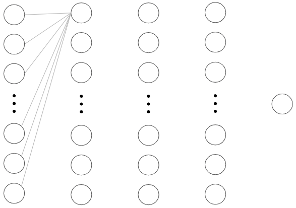
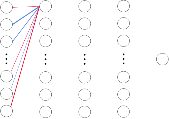
In the next image, I’ve singled out the weights connecting one neuron in the second layer to all the neurons in the previous layer. Each neuron acts like a function which outputs a value based on the input from all the neurons in the previous layer.
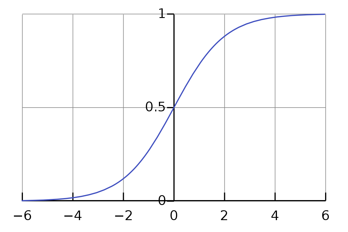
The actual function used for a neuron is called its activation function. To keep this demonstration simple and intuitive, we’ll have our neurons use the sigmoid function, which ensures that all outputs are between 0 and 1, regardless of the input value. As you can see in the diagram, large negative inputs result in an output around 0, while large positive values converge around an output of 1.
In case you’re wondering, the purpose of the activation function is to introduce non-linearity to the model. Without an activation function, the entire neural network would just be a linear regression model, because adding linear functions produces a linear function. A model without activation functions would not be able to make any complex associations. I’ll give a simple example below. Feel free to skim this part if it already makes sense to you.
A linear activation function can be represented in the form of y = mx + b, where ‘y’ represents the output of the neuron, ‘x’ represents the input, ‘b’ represents the bias, and ‘m’ represents the weight.
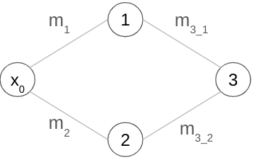
Let’s start by calling input to our network ‘x₀’. The equations of neurons 1 and 2 are respectively:
y₁ = m₁x₁ + b₁ || y₂ = m₂x₂ + b₂.
If we substitute the x values for with the input, ‘x’, our two equations become:
y₁ = m₁x₀ + b₁ || y₂ = m₂x₀ + b₂.
Next, the equation for neuron 3 can be represented as:
y₃ = m₃₁x₃₁ + b₃₁ + m₃₂x₃₂ + b₃₂
(The underscores have been omitted due to formatting issues)
If we substitute the equations from neurons 1 and 2 into the equation for the third neuron we get:
y₃ = m₃₁(m₁x₀ + b₁) + b₃₁ + m₃₂(m₂x₀ + b₂) + b₃₂
y₃ = m₃₁m₁x₀ + m₃₁b₁ + b₃₁ + m₃₂m₂x₀ + m₃₂b₂ + b₃₂
This looks like a mess right now, but remember since all the weights and biases, ‘m’ and ‘b’, are constants, they can simply be combined into one constant.
y₃ = (m₃₁m₁ + m₃₂m₂)x₀ + (m₃₂b₂ + m₃₁b₁ + b₃₁ + b₃₂ )
y₃ = mx₀ + b
When using linear activation functions, everything will collapse into one linear function regardless of how many layers or neurons there are. As you can see, it’d be much easier to just use a linear function to begin with.
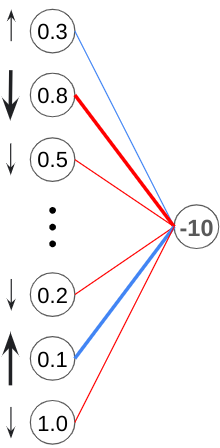
Moving on, we have weights. Weights act as a multiplier for the previous neuron’s output value before they are added to the next neuron’s input. Blue weights represent positive multipliers, while red weights represent negative multipliers. A thicker line represents a heavier weight, or in other words, a larger multiplier.
The weights are multiplied by the output values for each neuron, and all of them are added together and passed into the neuron in the next layer.
Mathematically, the input for this neuron can be represented as: (w₁a₁ + w₂a₂ + w₃a₃ + … + wₙaₙ), where “a” represents the activation/output value of the neuron in the previous layer, and “w” represents the weight connecting it to the neuron in the next layer. This is also known as the weighted sum.
Here’s an example which assumes the input layer only consists of 6 neurons:
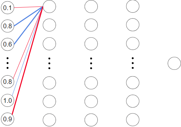
If we assume that a thicker line represents a x2 multiplier while a thinner line represents a x0.5 multiplier, then the weighted sum would be:
[(0.1 * -0.5) + (0.8* 2) + (0.6 * 2) + (0.8 * -0.5) + (1.0 * 0.5) + (0.9 * -2)] = 1.05
If we passed this value into the sigmoid activation function of the second layer neuron, we’d get an output value around 0.75.
At this point, you may be wondering what each output value of the first layer neurons even represent. Hang tight, we’ll get there soon!
Before we move on, there’s one more factor that influences the output value of a neuron. It’s bias, which is a constant that is added to the weighted sum of a neuron’s input before it’s processed.
With this new information, our weighted sum can be modelled as: (w₁a₁ + w₂a₂ + w₃a₃ + … + wₙaₙ + b), where “b” represents the bias.
You can think of bias as a neural network’s way of making adjustments that can’t be achieved by modifying the weights in a network. By modifying its weights and biases, a neural network is able to learn complex associations! We’ll go into the details of how it decides which weights and biases to increase or decrease later.
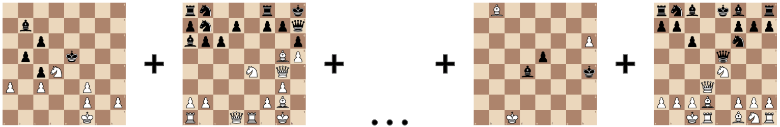
First, let’s go through an intuitive example of what each part of a trained neural network might do. Keep in mind that the function of neurons in a trained neural network is usually much more abstract than the examples we’ll be going into here.
For the purposes of our introductory article, we won’t be going into exactly what part of the chess board each input neuron represents, but usually, a chess position is fed into a neural network in the form of bitboards. I’ll represent the first layer as a board position since it’s much easier than trying to draw and explain a huge number of weights between the first and second layer neurons.
In our example, the second layer of the network might have neurons that are trained to fire for things like pawn islands, doubled pawns, how close the King is to the center of the board, or how many squares a Bishop has available to it.
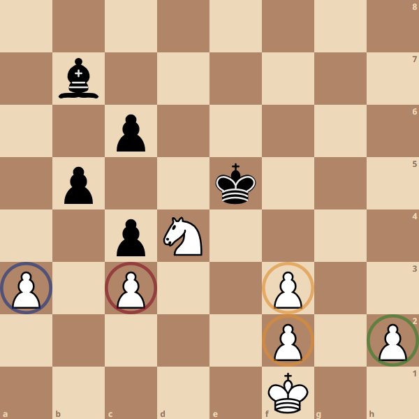
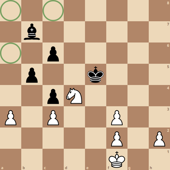
In a position like the image above, the neuron responsible for determining the quantity of pawn islands for white would output a value of 1, if we imagine an output of 0 indicating there are no pawn islands while an output of 1 corresponds to the maximum number of pawn islands possible (4 pawn islands)
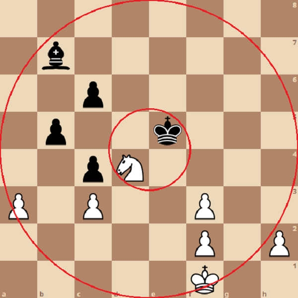
Meanwhile the neuron responsible for determining how close black’s King is to the center would output a value of 1, since it is as close to the center as possible, while the neuron responsible for determining white’s distance to the center would output a value closer to 0.
Finally, the neuron responsible for determining the quantity of bishop moves would give an output close to 0, where 0 is no possible bishop moves, and 1 is the maximum possible number of bishop moves (It can cover a maximum of 13 squares at once)
Keep in mind that neurons can only output a scalar quantity, so all individual neurons must represent quantifiable values.
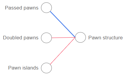
The next layer might have a neuron which combines information about pawn islands, doubled pawns, and passed pawns to give an evaluation for pawn structure. In this case, the weights for the passed pawn would likely be positive meaning it is good for the pawn structure, while the weights for the doubled pawns and pawn islands would likely be negative, since those features are bad for pawn structure. In our example, the outputs from the other neurons in the previous layer would have little to no impact on the pawn structure, therefore they are omitted from the illustration. This is rarely the case in real neural networks much more abstract connections
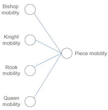
Another neuron in the second layer might combine information about how many legal moves each piece has to give an evaluation of piece mobility. If you’re knowledgeable about chess you’ll know there are many more factors that go into pawn structure and piece mobility than mentioned, but this is simplified for those who aren’t so into chess, so hush :)
In the third layer, a neuron might determine King safety by combining information such as the total number of opponent’s pieces left on the board and the mobility of those pieces, and how close the King is to the center of the board. Finally, the final neuron takes the outputs from all the third layer neurons and gives us a single number as the static evaluation for the board position.
The basic idea is that each layer builds on information from the previous layer, forming more complex concepts as we move through the network. In a way, each of the aspects we covered here form the basis for how a traditional chess engine works. Traditional chess engines are preprogrammed to recognize aspects of a position like piece development, king safety, and pawn structure, which help it provide a static evaluation of a position. These are known as heuristics.
Before the introduction of self learning AI to the chess community, these heuristics were designed and constantly tweaked by grandmasters to improve an engine’s performance. In a neural network evaluation, the network is able to get an intuitive feel of the evaluation based on similar past positions it has seen before, much like a human would.
In a way, the hidden layers create their own set of heuristics, and in the process, maybe come up with new heuristics that human grandmasters weren’t aware of. This is what gives neural networks more potential than traditional engines.
If you’d like to know how an engine uses its static evaluation function to determine what moves to make, be sure to stay tuned for my upcoming article on coding a chess engine using neural networks :)
The next big question is, how does a computer learn to make all these associations in the first place? After all, that’s at the core of what makes machine learning so powerful.
Here’s how it works.
A neural network is initialized with random weights and biases. So initially, when fed an position like this:
The output would be completely random.
In essence, what happens next is we tell the neural network how close its answer was to a “correct” evaluation, and the network then adjusts its weights and biases so that the next time it encounters the same position its output would be closer to the desired output.
There’s actually a few ways to tell a neural network the “correct” output. One way is to collect original data through self-play, and seeing which positions lead to wins or losses, like AlphaZero. The other way is to use existing game databases. Another approach uses the end result of games from a game database to get a rough idea whether a position was good or bad (the assumption is that, especially at the higher levels, a good position for one color generally leads to a win for that color). Alternatively, we can compare the board evaluation from a trusted engine to train our network. We’ll be using this last method in our example, since it is the most intuitive one to grasp.
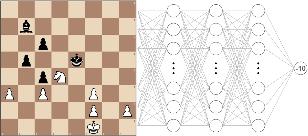
Back to our example. Imagine the neural network randomly decides that the position is -10 favouring black. Meanwhile, the Stockfish evaluation shows that in reality it is +4.5 in favour of white.
How far off the neural network is from the actual evaluation is represented in something called the cost function, where the difference between the desired and actual output are squared.
(4.5 — (-10))2 = 210.25
Squaring the difference places a much larger emphasis on big differences over small differences. This means if the neural network outputs a +2 instead of a +1, the network will be adjusted much less than if the network outputs a -10 instead of +4.5.
After determining the value of the cost function, the neural network will figure out a list of adjustments it needs to make to its weights and biases through a process known as backpropagation.
I’ll give a quick summary, but if anything’s unclear, feel free to dive deeper on your own.
There are three ways to adjust the output of this final evaluation neuron: Adjusting the biases, weights, and outputs of previous neurons
We only need to focus on the second to last layer for now.
Before we go on, I want to clarify that when I say “increase”, I mean making a number more positive, while “decrease” means to make a number more negative.
First, let’s cover the bias. This one’s pretty simple. Since we want the output to be more positive, we increase the value of the bias for the final neuron. This means a greater weighted sum which leads to a greater output value.
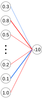
Next, let’s take a look at the weights. In this example, our output was too negative, we want to make all weights more negative. However, what’s important to notice is that the weights connected to greater output values (like this one with an output of 1.0), have a much greater impact than weights that are connected to neurons that barely fired (the ones with values close to 0). To maximize effectiveness, we want to focus more on changing the weights that are connected to neurons with greater outputs.
In this case, the weights connected to these neurons would be increased the most.
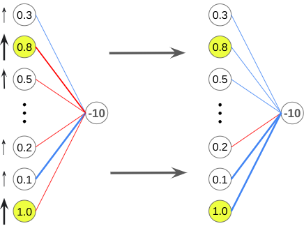
Finally, we have the outputs of the previous layer. Similar to how we changed the weights, we want to maximize effectiveness by focusing on the outputs that are weighted most heavily more than the ones connected to the final neuron by lighter weights.
However, we can’t change their outputs directly, so what do we do?
We modify the weights and biases of the previous layer! Using the list of desired changes we want to make to the second last layer (L-1), we can adjust the weights and biases linked to each of these neurons just like we did for the output layer. For the L-1 layer, instead of just accounting for the one neuron like the evaluation neuron, we want to repeat this process for every single neuron in the L-1 layer.
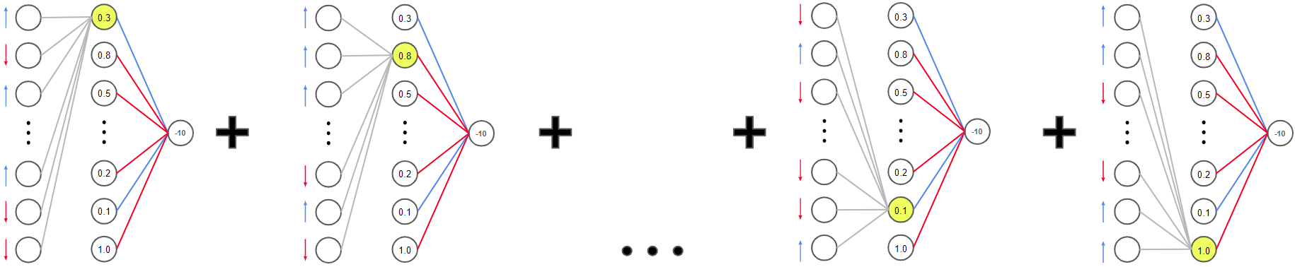
As you can see, each neuron in the L-1 layer wants the outputs in the previous layer to be changed in a different way, so the way we determine the final desired change for each neuron in the L-2 layer is to sum up all the desired changes.
The changes desired by neurons that require larger changes (the neurons with output values of 0.1 and 0.8 in the previous diagram) will have a larger influence than the other neurons.
We keep doing this for each layer until we propagate back towards the beginning of the neural network. Hence the term, “backpropagation”. We won’t be going into the math behind this, but the oversimplified version is that we use math to find the minimum of the cost function, where the variables of the cost function are all the weights and biases of the neural network. For anyone familiar with functions, that means at least tens of thousands of variables!
And of course, we can’t forget that all of this is just for a single position. Now, the same process is repeated for the rest of the positions in the training set, with each position nudging the network to make different changes to its weights and biases.
Finally, the average change suggested for each weight is applied, leaving us with a better neural network. This process is repeated until the neural network reaches a desired level of performance, or can no longer improve due to limited data or network complexity
To recap:
- Each layer of the neural network builds on the previous layer, increasing the complexity of concepts each neuron is responsible for as we move closer toward the output.
- During the training process, a neural network compares its output to the correct output, and creates a list of changes required for its weights and biases to try and get its output to be closer to the correct value.
- This process is repeated for each of the training examples/board positions, and the average change of for each weight and bias is applied to the network, leaving us with a better version.
- Training continues until a network reaches a desired level or its performance stagnates due to lack of data or a limited number of neurons and layers.
Now you know how a neural net-works :D
Before we reach the end of this article, I’d like to leave you with just a few thoughts on how intelligent game agents can be used in the future.
Imagine having a game where your AI companions can remember previous interactions and behave how you desire simply by receiving verbal instructions instead of having its behaviours linked to a fixed set of commands. What if the AI could even come up with and suggest its own ideas to you, much like how Meta’s Diplomacy AI suggested better moves to its human allies?
Maybe there’s a game that you feel like you’re no longer improving at, despite constant practice, and hours spent scrolling through forums searching for new strategy after strategy. If you’re not a professional gamer, chances are you don’t have a coach that has time to watch all your games and give reliable advice. However, a game agent that actually understood the game could play that role. It’d be able to analyze all of your gameplay and identify which changes you’d need to make to your gameplay to get the greatest return.
Another benefit of game agents is the speed at which they’d be able to playtest a game, since they could play many iterations in the time that a human could. All the balance issues and bugs would be discovered way before they started upsetting the gaming community.
Finally, we’d have intelligent companions or adversaries to play any game with, whether cooperative or competitive! No longer will there be an easy winning strategy like the ones that bug out hard coded AI. Nor will you have to worry about playing with friends who are too good or too bad for you when an AI can customize its level to give you the best experience possible. Wouldn’t that be amazing?
Sources
Neural networks (Amazing explanations!) https://www.3blue1brown.com/lessons/neural-networks